wCorr Arguments
Paul Bailey, Ahmad Emad, Ting Zhang, Qingshu Xie
2023-08-18
Source:vignettes/wCorrArguments.Rmd
wCorrArguments.RmdThe wCorr package can be used to calculate Pearson, Spearman, polyserial, and polychoric correlations, in weighted or unweighted form.1 The package implements the tetrachoric correlation as a specific case of the polychoric correlation and biserial correlation as a specific case of the polyserial correlation. When weights are used, the correlation coefficients are calculated with so called sample weights or inverse probability weights.2
This vignette describes the use of applying two Boolean switches in the wCorr package. It describes the implications and uses simulation to show the impact of these switches on resulting correlation estimates.
First, the Maximum Likelihood, or ML switch uses the
Maximum Likelihood Estimator (MLE) when ML=TRUE or uses a
consistent but non-MLE estimator for the nuisance parameters when
ML=FALSE. The simulations show that using
ML=FALSE is preferable because it speeds computation and
decreases the root mean square error (RMSE) of the estimator.
Second the fast argument gives the option to use a pure
R implementation (fast=FALSE) or an implementation that
relies on the Rcpp and RcppArmadillo packages
(fast=TRUE). The simulations show agreement to within \(10^{-9}\), showing the implementations
agree. At the same time the fast=TRUE option is always as
fast or faster.
In addition to this vignette, the wCorr Formulas vignette describes the statistical properties of the correlation estimators in the package and has a more complete derivation of the likelihood functions.
The ML switch
The wCorr package computes correlation coefficients between two vectors of random variables that are jointly bivariate normal. We call the two vectors X and Y.
\[\begin{pmatrix} X \\ Y \end{pmatrix} \sim N \left[ \begin{pmatrix} \mu_x \\ \mu_y \end{pmatrix}, \boldsymbol{\Sigma} \right] \]
where \(N(\mathbf{A},\boldsymbol{\Sigma})\) is the bivariate normal distribution with mean A and covariance \(\boldsymbol{\Sigma}\).
Computation of polyserial correlation
The likelihood function for an individual observation of the polyserial correlation is3
\[\mathrm{Pr}\left( \rho=r, \boldsymbol{\Theta}=\boldsymbol{\theta} ; Z=z_i, M=m_i \right) = \phi(z_i) \left[ \Phi\left( \frac{\theta_{m_i+2} - r \cdot z_i}{\sqrt{1-r^2}} \right) - \Phi \left( \frac{\theta_{m_i+1} - r \cdot z_i}{\sqrt{1-r^2}} \right) \right]\]
where \(\rho\) is the correlation between X and Y, Z is the normalized version of X, and M is a discretized version of Y, using \(\boldsymbol{\theta}\) as cut points as described in the wCorr Formulas vignette. Here an i is used to index the observed units.
The log-likelihood function (\(\ell\)) is then
\[\ell(\rho, \boldsymbol{\Theta}=\boldsymbol{\theta};\mathbf{Z}=\mathbf{z},\mathbf{M}=\mathbf{m}) = \sum_{i=1}^n w_i \ln\left[ \mathrm{Pr}\left( \rho=r, \boldsymbol{\Theta}=\boldsymbol{\theta} ; Z=z_i, M=m_i \right) \right]\]
The derivatives of \(\ell\) can be
written down but are not readily computed. When the ML
argument is set to FALSE (the default), the values of \(\boldsymbol{\theta}\) are computed using a
consistent estimator4 and a one dimensional optimization of \(\rho\) is calculated using the
optimize function in the stats package. When
the ML argument is set to TRUE, a
multi-dimensional optimization is done for \(\rho\) and \(\boldsymbol{\theta}\) using the
bobyqa function in the minqa package.
Computation of polychoric correlation
For the polychoric correlation the observed data is expressed in ordinal form for both variables. Here the discretized version of X is P and the discretized version of Y remains M.5 The likelihood function for the polychoric is
\[\mathrm{Pr}\left( \rho=r, \boldsymbol{\Theta}=\boldsymbol{\theta}, \boldsymbol{\Theta}'=\boldsymbol{\theta}' ; P=p_i, M=m_i \right) = \int_{\theta_{p_i+1}'}^{\theta_{p_i+2}'} \int_{\theta_{m_i+1}}^{\theta_{m_i+2}} \mkern-40mu f(x,y|\rho=r) dy dx\]
where \(f(x,y|r)\) is the normalized bivariate normal distribution with correlation \(\rho\), \(\boldsymbol{\theta}\) are the cut points used to discretize Y into M, and \(\boldsymbol{\theta'}\) are the cut points used to discretize X into P.
The log-likelihood is then \[\ell(\rho, \boldsymbol{\Theta}=\boldsymbol{\theta}, \boldsymbol{\Theta}'=\boldsymbol{\theta}' ;\mathbf{P}=\mathbf{p}, \mathbf{M}=\mathbf{m}) = \sum_{i=1}^n w_i \ln\left[\mathrm{Pr}\left( \rho=r, \boldsymbol{\Theta}=\boldsymbol{\theta},\boldsymbol{\Theta}'= \boldsymbol{\theta}' ; P=p_i, M=m_i \right) \right] \]
The derivatives of \(\ell\) can be
written down but are not readily computed. When the ML
argument is set to FALSE (the default), the values of \(\boldsymbol{\theta}\) and \(\boldsymbol{\theta}'\) are computed
using a consistent estimator and a one dimensional optimization of \(\rho\) is calculated using the
optimize function in the stats package. When
the ML argument is set to TRUE, a
multi-dimensional optimization is done for \(\rho\), \(\boldsymbol{\theta}\), \(\boldsymbol{\theta}'\) using the
bobyqa function in the minqa package.
Simulation study
To demonstrate the effect of the ML and
fast switches a few simulation studies are performed to
compare the similarity of the results when the switch is set to
TRUE to the result when the switch is set to
FALSE. This is done first for the ML switch
and then for the fast switch.
Finally, simulations show the implications of these switches on the speed of the computation.
General procedures of the simulation study of unweighted correlations
A simulation is run several times.6 For each iteration, the following procedure is used:7
- select a true correlation coefficient \(\rho\);
- select the number of observations \(n\);
- generate X and Y to be bivariate normally distributed using a pseudo-Random Number Generator (RNG);
- using a pseudo-RNG, select the number of bins for M and P (\(t\) and \(t'\)) independently from the set {2, 3, 4, 5};
- select the bin boundaries for M and P (\(\boldsymbol{\theta}\) and \(\boldsymbol{\theta}'\)) by sorting the results of \((t-1)\) and \((t'-1)\) draws, respectively, from a normal distribution using a pseudo-RNG;
- confirm that at least 2 levels of each of M and P are occupied (if not, return to the previous step); and
- calculate and record the correlation coefficients.
One of a few possible statistics is then calculated. To compare two levels of a switch the Relative Mean Absolute Deviation is used
\[RMAD= \frac{1}{m} \sum_{j=1}^m | r_{j, \mathtt{TRUE}} - r_{j, \mathtt{FALSE}} | \]
where there are \(m\) simulations
run, \(r_{j, \mathtt{TRUE}}\) and \(r_{j, \mathtt{FALSE}}\) are the estimated
correlation coefficient for the \(j\)th
simulated dataset when the switch is set to TRUE and
FALSE, respectively. This statistic is called “relative”
because it is compared to the other method of computing the statistic,
not the true value.
To compare either level to the true correlation coefficient the Root Mean Square Error is used
\[RMSE= \sqrt{ \frac{1}{m} \sum_{j=1}^m (r_j - \rho_j)^2 } \]
where, for the \(j\)th simulated dataset, \(r_j\) is an estimated correlation coefficient and \(\rho_j\) is the value used to generate the data (X, Y, M, and P).
ML switch
A simulation was done using the Cartesian product (all possible
combinations of) \(\mathtt{ML} \in
\{\mathtt{TRUE}, \mathtt{FALSE} \}\), \(\rho \in \left( -0.99, -0.95, -0.90, -0.85, ...,
0.95, 0.99 \right)\), and \(n \in \{10,
100, 1000\}\). Each iteration is run three times to increase the
precision of the simulation. The same values of the variables are used
in the computation for ML=TRUE as well as for
ML=FALSE; and then the statistics are compared between the
two sets of results (e.g. ML=TRUE and
ML=FALSE).
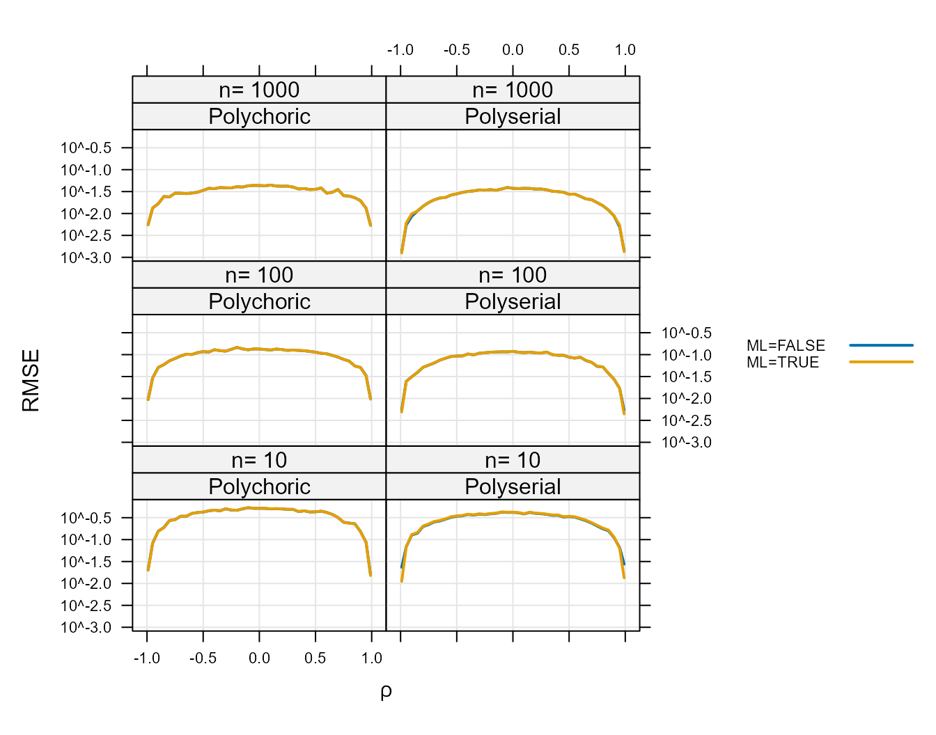
Figure 1 :. Root Mean Square Error for
ML=TRUE and ML=FALSE.
The RMSE for these two options is so similar that the two lines
cannot be distinguished for most of the plot. The exact differences are
shown for Polychoric in Table 1 : and for Polyserial in Table 2 :. The
column labeled, “RMSE difference” shows how much larger the RMSE is for
ML=TRUE than ML=FALSE. Because this difference
is always positive the RMSE of the ML=FALSE option is
always lower. Because of this the ML=TRUE option is
preferable only in situations where there is a reason to prefer MLE for
some other reason.
Table 1 :. Relative Mean Absolute Deviation
between ML=TRUE and ML=FALSE for
Polychoric.
| Correlation type | n | RMSE ML=TRUE | RMSE ML=FALSE | RMSE difference | RMAD |
|---|---|---|---|---|---|
| Polychoric | 10 | 0.1585 | 0.1571 | 0.0013 | 0.1585 |
| Polychoric | 100 | 0.0112 | 0.0112 | 0.0000 | 0.0112 |
| Polychoric | 1000 | 0.0011 | 0.0011 | 0.0000 | 0.0011 |
Table 2 :. Relative Mean Absolute Deviation
between ML=TRUE and ML=FALSE for
Polyserial.
| Correlation type | n | RMSE ML=TRUE | RMSE ML=FALSE | RMSE difference | RMAD |
|---|---|---|---|---|---|
| Polyserial | 10 | 0.3155 | 0.3098 | 0.0057 | 0.3155 |
| Polyserial | 100 | 0.0866 | 0.0864 | 0.0002 | 0.0866 |
| Polyserial | 1000 | 0.0273 | 0.0273 | 0.0000 | 0.0273 |
For the Polychoric, the agreement between these two methods, in terms of MSE is within 0.001 for \(n\) of 10 and decreases to within less than 0.0000 for \(n\) of 100 or more. Given the magnitude of these differences the faster method will be preferable.
The final column in the above tables shows the RMAD which compares
how similar the ML=TRUE and ML=FALSE results
are to each other. Because these values are larger than 0, they indicate
that there is not complete agreement between the two sets of estimates.
If a user considers the MLE to be the correct estimate then they show
the deviation of the ML=FALSE results from the correct
results.
fast switch
This section examines the agreement between the pure R implementation
of the function that calculates the correlation and the
Rcpp and RcppArmadillo implementation, which
is expected to be faster. The code can compute with either option by
setting fast=FALSE (pure R) or fast=TRUE
(Rcpp).
A simulation was done at each level of the Cartesian product of \(\mathtt{fast} \in \{\mathtt{TRUE}, \mathtt{FALSE}
\}\), \(\rho \in \left( -0.99, -0.95,
-0.90, -0.85, ..., 0.95, 0.99 \right)\), and \(n \in \{10, 100, 1000\}\). Each iteration
was run 100 times. The same values of the variables are used in the
computation for fast=TRUE as well as for
fast=FALSE; and then the statistics are compared between
the two sets of results.
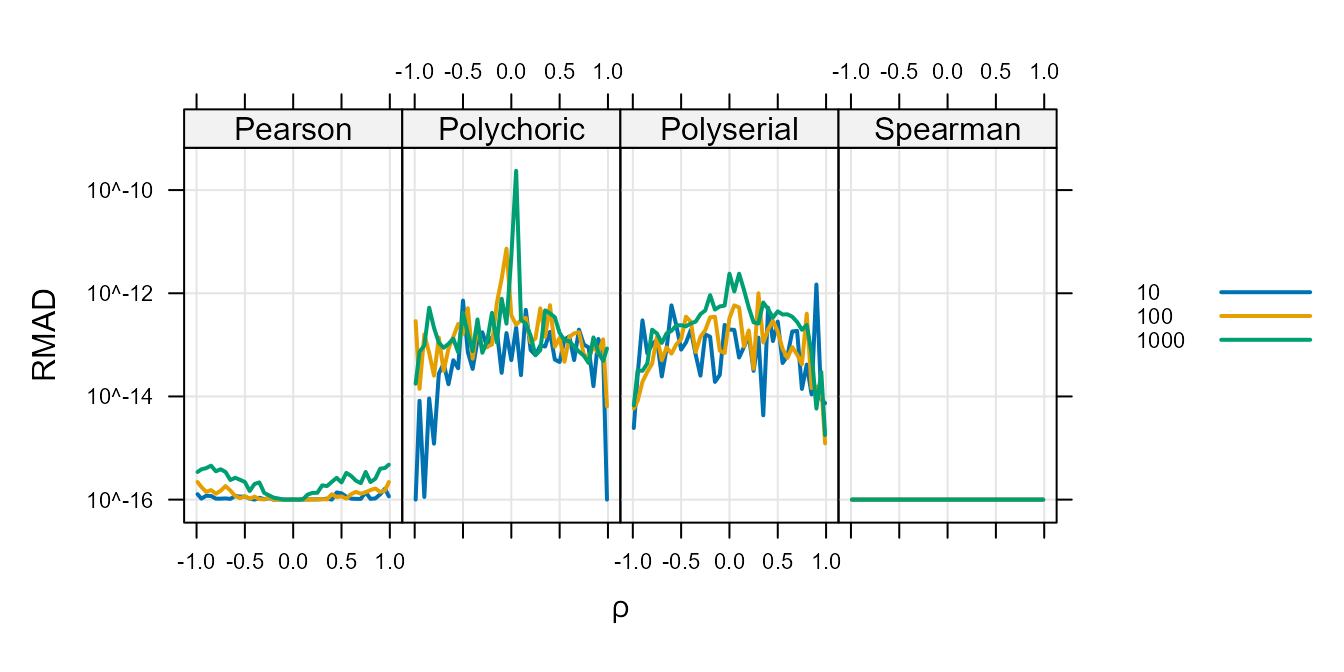
The plot below shows all differences between the
fast=TRUE and fast=FALSE runs for the four
types of correlations. Note that differences smaller than \(10^{-16}\) are indistinguishable from 0 by
the machine. Because of this, all values were shown as being at least
\(10^{-16}\) so that they could all be
shown on a log scale.
Figure 2 :. Relative Mean Absolute Differences
between fast=TRUE and fast=FALSE.
The above shows that differences as a result of the fast
argument are never expected to be larger than \(10^{-9}\) for any type or correlation type.
The Spearman never shows any difference that is different from zero and
the Pearson show differences just larger than the smallest observable
difference when using double precision floating point values (about
\(1 \times 10^{-16}\)). This indicates
that the computation differences are completely irrelevant for these two
types.
For the other two types, it is unclear which one is correct and the
agreement that is never more distant than the \(10^{-9}\) level indicates that any use that
requires precision of less than \(10^{-9}\) can use the
fast=TRUE argument for faster computation.
Implications for speed
To show the effect of the ML and fast
switches on computation a simulation was done at each level of the
Cartesian product of \(\mathtt{ML} \in
\{\mathtt{TRUE}, \mathtt{FALSE} \}\), \(\mathtt{fast} \in \{\mathtt{TRUE}, \mathtt{FALSE}
\}\), \(\rho \in \left( -0.99, -0.95,
-0.90, -0.85, ..., 0.95, 0.99 \right)\), and \(n \in \{10^1, 10^{1.25}, 10^{1.5}, ...,
10^7\}\). Each iteration is run 80 times when \(n<10^5\) and 20 times when \(n\geq 10^5\). The same values of the
variables are used in the computations at all four combinations of
ML and fast. A variety of correlations are
chosen so that the results represent an average of possible values of
\(\rho\).
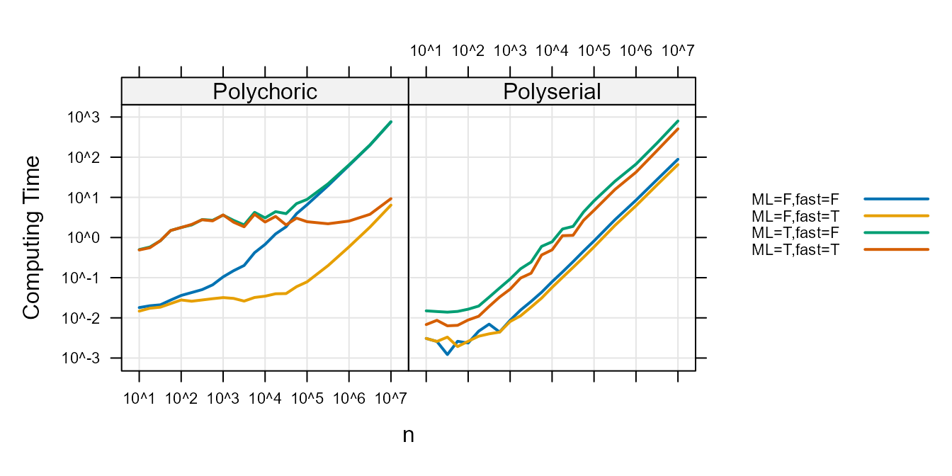
The following plot shows the mean computing time (in seconds) versus \(n\).
Figure 3 :. Computation time
comparison.
In all cases setting the ML option to FALSE
and the fast option to TRUE speeds up–or does
not slow down computation. Users wishing for the fastest computation
speeds will use ML=FALSE and fast=TRUE.
For the Polychoric, when \(n\) is a
million observations (\(n=10^7\)), the
speed of a correlation when fast=FALSE is 761 seconds and
when the fast=TRUE it is and 8 seconds. When
fast=TRUE, setting ML=FALSE speeds computation
by 3 seconds.
For the Polyserial, when \(n\) is a
million observations, the speed of a correlation when
ML=TRUE is 652 seconds and when the ML=FALSE
it is and 77 seconds. When ML=FALSE, setting
fast=TRUE speeds computation by 24 seconds.
#Conclusion Overall the simulations show that the ML
option is not more accurate but does add computation burden.
The fast=TRUE and fast=FALSE option are a
Rcpp version of the correlation code and an R
version, respectively and agree with each other–the differences are not
expected to be larger than \(10^{-9}\).
Thus users wishing for fastest computation speeds and accurate
results can use ML=FALSE and fast=TRUE.
The estimation procedure used by the wCorr package for the polyserial is based on the likelihood function in by Cox, N. R. (1974), “Estimation of the Correlation between a Continuous and a Discrete Variable.” Biometrics, 30 (1), pp 171-178. The likelihood function for polychoric is from Olsson, U. (1979) “Maximum Likelihood Estimation of the Polychoric Correlation Coefficient.” Psyhometrika, 44 (4), pp 443-460. The likelihood used for Pearson and Spearman is written down many places. One is the “correlate” function in Stata Corp, Stata Statistical Software: Release 8. College Station, TX: Stata Corp LP, 2003.↩︎
Sample weights are comparable to
pweightin Stata.↩︎See the wCorr Formulas vignette for a more complete description of the polyserial correlations’ likelihood function.↩︎
The value of the nuisance parameter \(\boldsymbol{\theta}\) is chosen to be \(\Phi^{-1}(n/N)\) where \(n\) is the number of values to the left of the cut point (\(\theta_i\) value) and \(N\) is the number of data points overall. For the weighted cause \(n\) is replaced by the sum of the weights to the left of the cut point and \(N\) is replaced by the total weight of all units. See the wCorr Formulas vignette for a more complete description.↩︎
See the “wCorr Formulas” vignette for a more complete description of the polychoric correlations’ likelihood function.↩︎
The exact number is noted for each specific simulation.↩︎
When the exact method of selecting a parameter (such as \(n\)) is not noted above, it is described as part of each simulation.↩︎